ILPs for Blocked n-Queens

In this post I’ll go through both ILP (Integer Linear Programming) frameworks that I developed while working on the blocked n-Queen problem. Click here to play the game, or here to read the main article on the topic.

Base Model

The goal of the base model is to take an n-W board configuration and find its value and an optimal solution as quickly as possible. It needs to be able to efficiently run through many board configurations in order to collect boards and solutions.

In order to do that, I wrote it so that the added complexity of the walls is moved to the model building part rather than encoded within the ILP itself. The idea is to try to make the complexity of the ILP about equal to the classic n-Queen problem, which is known to be solved very fast.

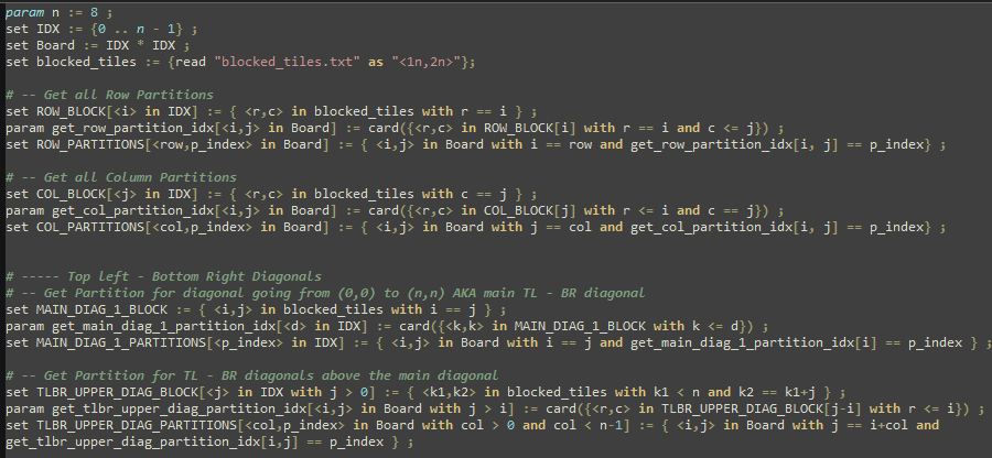
Let’s look at some of the zimpl code. The totality of it can be found in the GitHub repository.

param n := 8 ;
set IDX := {0 .. n - 1} ;
set Board := IDX * IDX ;
set blocked_tiles := {read "blocked_tiles.txt" as "<1n,2n>"};

We start by initializing some basic parameters and sets. n is the board size, which is hard-coded as 8. As described in the main article, a board is simply a set of tuples representing coordinates on the board. The set of walls or blocked tiles is imported from a text file, in order to be easily modifiable from code. This feature is for example used when running the base model for all 2-W or 3-W boards – a loop ran through all the possible combinations (grouped by symmetry), modified the blocked tiles file, and ran the BM.

var QUEEN[Board] binary ;

maximize obj: sum <i,j> in Board: QUEEN[i,j] ;

The only variables in the model are the QUEEN variables. They are indexed by coordinates on the board, and are binary – a 1 means that a queen is present in that tile, a 0 that it isn’t. The objective function of the ILP is simply maximizing the number of queens.

Let’s see how the added complexity of the walls is actually handled by looking at the queen legality constraints for the rows.

set ROW_BLOCK[<i> in IDX] := { <r,c> in blocked_tiles with r == i } ;
param get_row_partition_idx[<i,j> in Board] := card({<r,c> in ROW_BLOCK[i] with r == i and c <=  j}) ;
set ROW_PARTITIONS[<row,p_index> in Board] := { <i,j> in Board with i == row and get_row_partition_idx[i, j] == p_index} ;

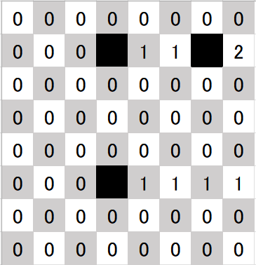
Each row is partitioned into k+1 sets, where k is the number of walls in that row. This is done by taking a coordinate (i, j), and simply counting how many walls there are in the the i-th row before the j-th column. Here’s a visual representation of what those params and sets do:

subto ROW_SAFE:
	forall <row, p_index> in Board:
		sum <i,j> in ROW_PARTITIONS[row, p_index]: QUEEN[i,j] <= 1 ;

The only constraint is that for each row, only 1 queen can be placed per partition set. In the example above, the top row can only have 1 queen in it, as there are no walls. The second row has 3 partition sets, as it has 3 walls. There can be at most 1 queen per partition set – for a total maximum of 3 in that row, each queen in its respective set.

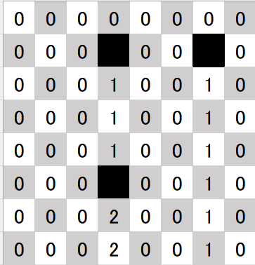
The same approach is taken for columns and diagonals. The code is the same with some index arithmetic tinkering. Here’s the column partition sets of the same board as above:

Solution-Counting Base Model

The BM stops looking for solutions as soon as it finds an optimal one, which makes sense for our purpose. But in order to count the solutions for an n-W board with a known value, we can simply remove the objective function and turn it into an equality constraint. This way, any feasible solution is actually an optimal solution of the original problem.

subto OBJ:
    sum <i,j> in Board: QUEEN[i,j] == value ;

Then, we modify the SCIP settings to count as many solutions as we want. I used this to filter out non-unique solutions in my search for interesting puzzles – I set it to count up to 2 solutions. If it finds 2, then it means that the board doesn’t have a unique optimal solution for its value.

Least Walls Model

The LWM is a modification of the base model that has the objective of finding the least amount of walls that are required in order to be able to fit q queens in a board. In other words, finding the smallest n such that an n-W board exists with value q.

In order to do so, we add a new parameter, some variables and some constraints:

param q := 11 ;

var BLOCKED[Board] binary ;
minimize obj: sum <i,j> in Board: BLOCKED[i,j] ;

subto QUEEN_COUNT:
    sum <i,j> in Board: QUEEN[i,j] == q ;

The set partitioning from the base model is scrapped, and the blocked tiles are modelled as variables, since we have no pre-existing knowledge of what the blocked tile set will look like for some value q.

Since we no longer have a set partitioning, the queen legality constraints are slightly more complicated. We can look at the row legality again:

subto ROW_SAFETY:
    forall <row> in IDX:
        forall <col1,col2> in Board with col1 < col2: 
            (sum <k> in IDX with k >= col1 and k <= col2: QUEEN[row,k]) <= 1 + (sum <k> in IDX with k > col1 and k < col2: BLOCKED[row,k]) ;

Let’s break it down for an example row – row 0. It takes a pair of columns col1 and col2, with col1 being smaller than col2. Then, it counts the number of queens in positions (0,k), where k is a column value between col1 and col2. Intuitively, if there are w walls in those (0,k) positions, you should be able to place w+1 queens, just like we saw for the base model. So the number of queens in (0, k) positions must be smaller or equal to the number of walls in those positions, plus one.

This is done for every (col1,col2) pair for every row, guaranteeing row safety in the board. The same logic is used for columns and diagonals.

Solution-Counting Least Walls Model

Just like for the base model, it’s easy to make a modification in order to count optimal solutions. Basically, once we know that q queens need at least w walls, we can check how many w-W boards exist that have value q.

subto OBJ:
    sum <i,j> in Board: BLOCKED[i,j] == w ;

subto QUEEN_COUNT:
    sum <i,j> in Board: QUEEN[i,j] == q ;